The logistic distribution, also known as the sigmoid distribution, is a continuous probability distribution in Python’s NumPy library.

Logistic Distribution is used to describe growth.

Used extensively in machine learning in logistic regression, neural networks etc.

It’s modeled by the numpy.random.logistic function and is useful for representing S-shaped curves where the probability of an event increases or decreases towards zero at either end of the distribution.

Here’s a breakdown of the logistic distribution and its implementation in NumPy:

Properties:

Represents a symmetrical S-shaped curve.
Range extends from negative infinity to positive infinity, but most probable values cluster around the location parameter (loc).

Parameters:

loc (float, optional): mean, where the peak is. The location parameter (default: 0) representing the inflection point of the S-shaped curve. The distribution is centered around this value.

scale (float, optional): standard deviation, the flatness of distribution. The scale parameter (default: 1) controlling the spread of the distribution. A larger scale leads to a gentler curve, while a smaller scale creates a steeper curve.

size – The shape of the returned array.

Applications:

Logistic regression: Modeling the probability of a binary outcome (e.g., success/failure, alive/dead) based on independent variables.
Machine learning: Used in various algorithms like neural networks for activation functions.
Simulating growth processes: Can represent logistic growth curves where the rate of change slows over time.

Example

from numpy import random

x = random.logistic(loc=1, scale=10, size=(2, 3))

print(x)

Output

[[ 20.90215077   1.19481827 -20.18975946]
 [ 17.57607324   5.445727    14.17197954]]

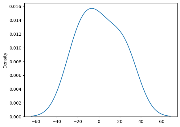
Visualization of Logistic Distribution

from numpy import random
import matplotlib.pyplot as plt
import seaborn as sns

sns.distplot(random.logistic(loc=1, scale=10, size=(2, 3)), hist=False)

plt.show()

Output